ranton.org - Building a Graph Algorithm Library with an AI Coding Agent

May 15, 2026

Introduction

This article walks through how I specified a non-trivial Rust graph library and then used an autonomous coding agent to build it inside a locked-down sandbox I’ve been building to better secure coding agents. I will walk through what worked, what broke, and what I’d change next time. The project itself is graphalglib, a from-scratch implementation covering foundational algorithms, visualization, simulated annealing, and genetic algorithms.

I’ve been working on a sandbox to run coding agents in while keeping access to the outer filesystem, host kernel, network, and any secrets locked down (more in AI Fortress, Part 2). I wanted a non-trivial task to validate the sandbox.

Starting with a good spec, pre-vendoring dependencies, and adding a HEAD-diff sanity check did most of the work. The failures clustered around missing function signatures in task descriptions and a poorly tuned GA. None of that’s surprising, but it’s worth seeing how those generic-sounding lessons land when applied to a real project.

This is mainly for people experimenting with agentic coding workflows, or anyone wondering how far you can push an LLM inside a hard sandbox with no network.

The Sandbox: AI Fortress and code-workers

The agent runs inside AI Fortress, a multi-layer sandboxing system I built to run AI coding agents safely on my workstation. It uses five layers of isolation:

Layer 0 (host): The Bifrost LLM gateway handles all upstream API calls and brokers multiple providers (Anthropic and OpenAI). The real provider keys never enter the VM. A dedicated UID plus nftables egress rules contain the process even if it’s compromised.
Layer 1 (KVM VM): A Flatcar Container Linux VM runs under KVM. The project directory is shared into the VM via a virtio-fs mount, so any file the agent writes lands directly on my host filesystem. No push, no pull, no sync layer.
Layer 2 (gVisor): The agent process itself runs inside a gVisor (runsc) container, which interposes a user-space kernel and intercepts all syscalls.
Layer 3 (network isolation): The container sits on an --internal Docker bridge with no default route and no NAT. There is no direct internet access from inside the sandbox.
Layer 4 (virtual key): Each session gets a fresh, budget-capped token (sk-bf-...) minted by the host. The cap was $5 per 8 hours. The real key never reaches the sandbox.

The no-internet constraint is the most important one from a project design perspective. It meant I had to pre-vendor all Rust dependencies before starting, and it ruled out any task that required fetching data at runtime. Everything the agent needed had to already be on disk.

Task dispatch was handled by code-workers, a pull-based orchestration layer I built alongside AI Fortress. A long-running worker container inside the sandbox long-polls a host-side FastAPI coordinator (bound to 127.0.0.1:7222). When a task arrives, worker.py executes it by invoking opencode (a CLI runner for coding agents) with a structured prompt, then posts the exit code and output tail back to the coordinator. On the host side, send_task.sh and poll_task.sh give a top-level orchestrator a simple interface for dispatching work and tracking status.

Work items were tracked with beads, a lightweight git-native issue tracker. Issues live as JSONL in .beads/issues.jsonl inside the repo. The key primitive for orchestration is bd ready, which returns all open issues with no unresolved dependencies. That’s exactly what you need when you’re running a dispatch loop and don’t want to reason about ordering yourself.

Picking the Right Project

Not every project is a good fit for autonomous agent development in a sandboxed environment. I had three hard constraints going in:

No internet access. Datasets and dependencies had to be pre-loaded.
No frontend. The agent can’t run a browser or interact with a UI.
Results have to be validatable. Not necessarily provably optimal, but checkable against known solutions or measurable against quality metrics.

For this phase of work — brainstorming and writing the spec — I used Perplexity.

I considered a range of candidates: compression algorithm suites, constraint satisfaction solvers, bytecode VMs, Monte Carlo game engines. The graph algorithm library stood out because it uniquely satisfied all three constraints. Foundational graph algorithms like BFS, Dijkstra, and Tarjan’s SCC are deterministically correct and easy to unit test. Optimization problems like graph coloring and TSP have well-established public benchmarks (DIMACS and TSPLIB) with known optimal or best-known solutions, which makes quality scoring straightforward.

Building the Specification

Once the graph library emerged as the best fit, the next step was to pin down a spec detailed enough that an agent could execute it autonomously. I wrote it through a series of focused conversations before writing any code. The goal was a document detailed enough that a beads issue could be seeded mechanically from each milestone, without any judgment calls left to the dispatch loop.

Algorithm Scope

The library would cover three categories.

First, foundational algorithms implemented correctly from scratch: BFS, DFS, Dijkstra, Bellman-Ford, Floyd-Warshall, Kruskal’s MST, Prim’s MST, Tarjan’s SCC, topological sort, cycle detection, and Edmonds-Karp max flow. These have deterministic correct outputs on any given input, making them straightforward to unit test against hand-crafted cases and cross-validate against each other.

Second, optimization heuristics in three phases: greedy baselines in Phase 1, simulated annealing in Phase 3, and genetic algorithms in Phase 4. The optimization problems were graph coloring, TSP, vertex cover, and maximum clique. All four have public benchmark datasets and known solutions to compare against.

Third, visualization in Phase 2: DOT and GraphML export with solution annotations, plus round-trip validation — export the graph with an algorithm’s output highlighted, parse it back, and verify the annotations match.

Three Graph Representations

One decision worth calling out: I specified three graph representations rather than the conventional two. Most algorithm texts cover adjacency lists and adjacency matrices. I added a third, the adjacency hashset.

The adjacency hashset is often the best practical trade-off for sparse graphs. It gives you O(1) edge existence checks (which a plain list doesn’t) while staying memory-efficient for sparse graphs (which a matrix doesn’t). In practice it ends up being the default representation for most algorithms, and I wanted the library to reflect that rather than defaulting to whichever structure textbooks happen to lead with.

Development Order and Validation Strategy

I wanted breadth-first development with depth-first validation: build the basics before the advanced stuff, but each algorithm has to be fully validated before moving on to the next. No partial implementations sitting around in the codebase waiting to be finished.

I also specified two distinct validation modes. A quick correctness suite runs after every algorithm implementation and must finish in under 10 seconds. It covers the unit tests and property checks for the new algorithm plus regression tests for everything already implemented. A full validation suite runs at phase boundaries and can take 5 to 30 minutes. It covers scaling benchmarks on graphs from 10 to 10,000 vertices, full DIMACS and TSPLIB benchmark runs, and optimization quality comparisons across approaches.

Visualization was treated as a phase gate. Not required in Phase 1, but once it was introduced in Phase 2, every subsequent feature had to include it. And validating visualization meant more than checking that it renders — it meant parsing the generated DOT or GraphML output and verifying the annotations are structurally correct. For a shortest path, the highlighted edges should form a connected path. For a graph coloring, the colored vertices should form independent sets. The agent had to prove the visualization was right, not just that it existed.

Language and Project Structure

Rust was the natural choice for me. Graph algorithms at scale need performance and precise memory management, and Rust’s type system and borrow checker give you correctness guarantees that are genuinely useful when you’re implementing a dozen related algorithms that all need to agree on the same graph representation.

The workspace was organized into three crates: graph-core for the library, graph-cli for a command-line interface, and graph-eval for the benchmarking harness. External crates were allowed for utilities — random number generation, serialization — but not for algorithm implementations. No petgraph. The full dependency set was pre-vendored (107 MB, 115 crates) into the repository before any agent dispatch, since the sandbox has no internet access. All subsequent cargo calls ran with --offline.

In a more complete system, I would want a pre-approved list or some other policy for what packages could be installed via the network control layer or a specialized tool provided to the agent in the sandbox. There would also be a mechanism to ask for approval of new packages so you don’t have to pre-install everything you might need. But for now I was more interested in testing whether the agent could keep looping autonomously on a bigger project. After all, if you can’t leave the agent to work independently for a while, automating package approval has less value.

Testing used Rust’s built-in #[test] framework with Criterion for benchmarks. Batch validation produced JSON output for programmatic analysis and markdown summaries for human review. Stochastic algorithms accepted an RNG seed for reproducibility. Error handling used Result and ? propagation throughout the library; panics were acceptable only in test and benchmark code.

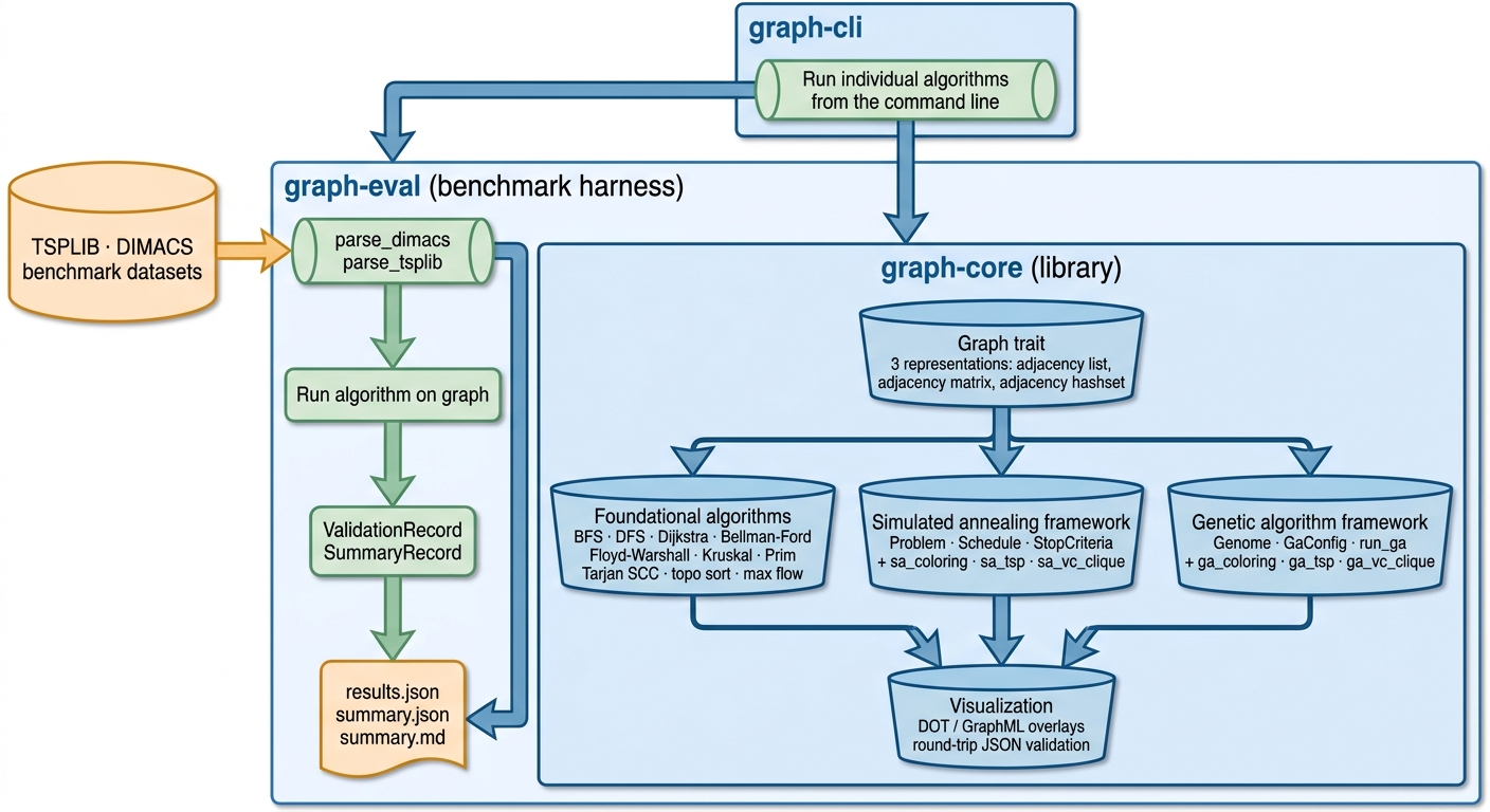
graph<em>alg</em>lib architecture: three Rust crates (graph-cli, graph-eval, graph-core), with graph-core containing the Graph trait and three algorithm buckets (foundational, simulated-annealing, genetic-algorithm) flowing into a shared visualization layer; graph-eval parses TSPLIB and DIMACS datasets and emits validation and summary records.

Above: how the pieces fit together. graph-core is the library; graph-cli and graph-eval are thin layers on top. Inside graph-core, the Graph trait sits underneath three algorithm categories — foundational, simulated annealing, genetic algorithm — that all feed a shared visualization layer. graph-eval parses TSPLIB and DIMACS datasets, runs the algorithm, and emits the JSON and markdown records the benchmark figures later in this article are built from.

Running the Agentic Build Loop

To actually build things, I used Claude Code with Opus 4.7 as the top-level orchestrator. Its job was to read the spec, file tasks into beads, and dispatch each one to the sandboxed coding agent via the send_task.sh script. Inside the sandbox, opencode ran the task, calling OpenAI GPT-5.3 through Bifrost.

The top-level orchestrator really doesn’t need permissions to do anything other than read the spec, commit results from the agent runs, and use beads to break up the work and track it.

With the spec finalized, I seeded (via Claude Code) 43 beads issues (gal-1 through gal-43) from the milestone structure, encoding dependency relationships with the --deps flag so bd ready would always return the correct next task. Four phase-level epics (gal-1, gal-23, gal-27, gal-33) served as umbrella trackers for the major phases.

The bootstrap step happened on the host before any agent dispatch. I initialized the Cargo workspace, ran cargo vendor, and committed the resulting vendor/ directory (107 MB, 115 crates) along with a .cargo/config.toml directing all subsequent builds to the local vendor tree. This was a prerequisite, not an optimization. Without it, every task dispatch would have required internet access and every cargo build would have failed inside the sandbox.

The dispatch loop for each task looked like this: mark the issue in-progress, record the current git HEAD, build a structured prompt from the issue title, description, and acceptance criteria, send it via send_task.sh --wait, and once the result came back, compare HEAD again.

The HEAD-diff check turned out to be the load-bearing piece. On one task the agent returned STATUS: DONE with a plausible-sounding commit message, but git HEAD hadn’t moved. The check caught it instantly and prevented a cascade of silent failures. If you’re running a similar loop, add this check.

Inside the sandbox, worker.py leased the task from the coordinator shim, invoked opencode run with the structured prompt, and streamed output back. Each opencode invocation was a fresh agent process. Most tasks completed in 3 to 8 minutes.

Sharp Edges

A few tasks needed intervention. The pattern I saw most often was BLOCKED responses citing missing context; the agent knew what it needed to do but couldn’t find the right API surface to work against. The fix was straightforward: edit the beads issue description to paste in the exact function signatures and module paths from the existing code. Once the brief read like “edit crates/graph-core/src/sa.rs — the existing trait is Problem, defined as…”, retries landed on the first attempt.

One task hit a different failure mode: the agent wrote good code but left three type errors it couldn’t resolve across two retries. Rather than dispatch a third time, I made the five edits directly on the host in about 30 seconds. The heuristic I settled on: if the sandbox returns BLOCKED twice on a compile-shaped failure, fix it locally. The agent’s time is better spent on the next task.

The TSPLIB canonical URL (comopt.ifi.uni-heidelberg.de/software/TSPLIB95/) returned a 404 over HTTPS during the session. I updated scripts/fetch_data.sh to use a GitHub mirror instead. This kind of thing is easy to miss until you actually run the data fetch.

Benchmark Results

The build session closed all 43 beads issues and produced 37 commits on main: 33 from the sandbox worker, 4 from the host. The workspace has 3 crates, and 49 tests pass under cargo test --workspace --offline.

The real benchmark results came from running the graph-eval binary against TSPLIB and DIMACS instances. For TSP, simulated annealing beats nearest-neighbor on every instance. The gaps to the known optimum were roughly 6–18% for SA versus 19–23% for nearest-neighbor — a meaningful improvement, consistent with what the spec predicted. The genetic algorithm underperformed nearest-neighbor at the default budget of 50 individuals over 200 generations. That’s a tuning problem, not a correctness problem, and it’s the obvious next knob to turn.

For graph coloring on queen5_5, greedy used 7 colors while both SA and GA found the chromatic number of 5, matching the known benchmark optimum for that family of instances. That’s the textbook case where stochastic search beats greedy, and it was good to see it show up in the actual benchmark output.

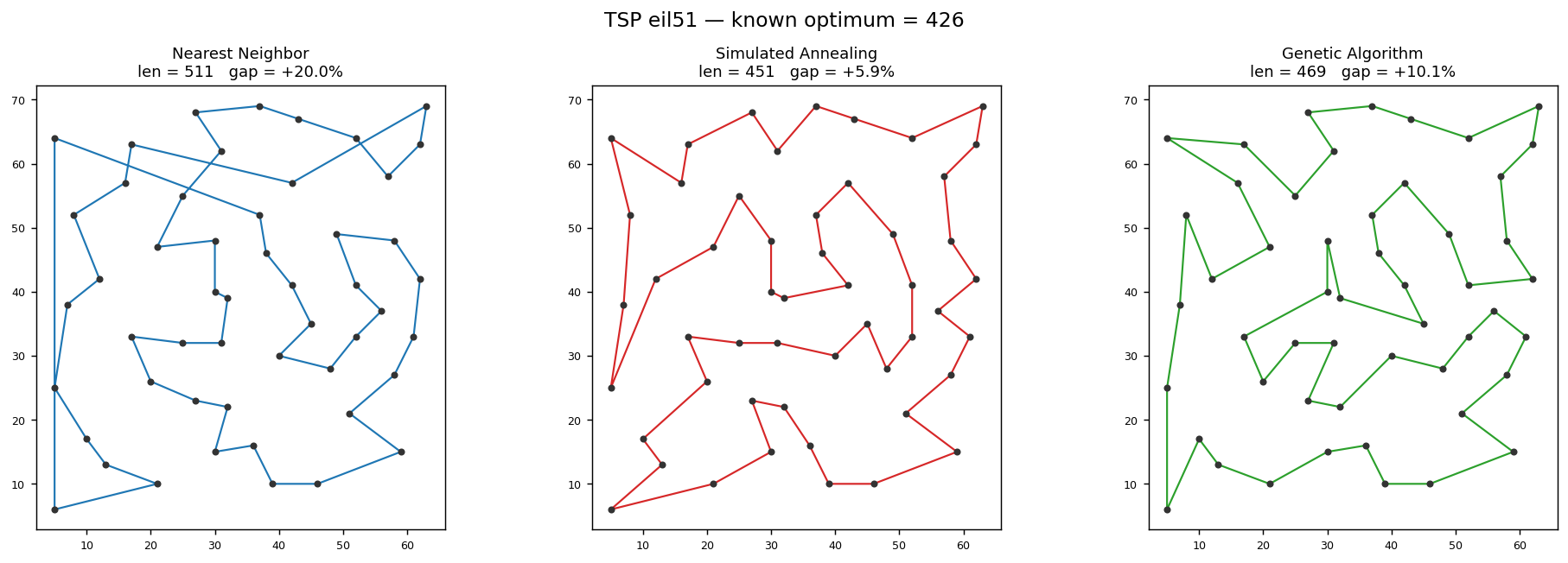
TSP eil51 solved with nearest-neighbor, simulated annealing, and a genetic algorithm, alongside the known optimal tour.

Above: TSP eil51 (TSPLIB benchmark, known optimum 426) solved with the three optimizer families. Nearest-neighbor gives a fast +20% baseline; simulated annealing closes most of the gap (+5.9%) with visibly fewer crossings; the genetic algorithm lands in between. All three runs are seeded and reproducible.

Instance	Method	Gap to optimum
eil51	Nearest-neighbor	~+20%
eil51	Simulated annealing	~+5.9%
eil51	Genetic algorithm	Between NN and SA

Costs

The whole project — 43 beads issues, 37 git commits, 4 phases of algorithms, documentation, real benchmarks — cost about $5.83. The cache-hit ratio is the dominant reason: 12.5M of 13.7M input tokens were cached_read_tokens, about 91%. This also shows Bifrost is propagating cache markers correctly.

There are some loose ends worth noting. The Phase 2 and Phase 3 batch artifact functions exist in the codebase but aren’t wired into main() — about 5 lines of plumbing. The DIMACS and TSPLIB dataset paths are hardcoded rather than read from datasets.toml because the toml crate wasn’t in the vendored set. These are small, well-scoped follow-up tasks that can go straight back into the same dispatch pipeline.

Lessons for Agentic Coding Workflows

A few things stand out from this process that I think apply generally to agentic coding workflows:

Spec granularity is the multiplier. The most important property of the specification is the acceptance criteria. Because each milestone had explicit, verifiable conditions, the agent had a concrete definition of done and a concrete pass/fail signal. A spec that says “implement Dijkstra’s algorithm” is much harder to dispatch than one that says “distances and reconstructed paths match known results on small graphs; cross-check against Bellman-Ford.”

Pre-vendoring is a prerequisite. Without offline-capable dependencies the sandbox’s network isolation makes every build fail. Ultimately, if the sandbox lives on to become more general-purpose, it’ll need a way to request and install approved packages — or trigger human-in-the-loop approval for them.

Task size matters as much as content. Tasks scoped to one source file with a small number of new tests landed on the first attempt in almost every case. Broader tasks that referenced existing APIs without providing exact signatures came back BLOCKED. The milestone structure in the spec naturally produced well-scoped tasks, which is one reason it worked as well as it did.

Verify independently. Don’t trust the agent’s self-reported status. The HEAD-diff check is two lines and it caught one silent failure that would otherwise have cascaded into the next task. Add it to your dispatch loop. Having a top-level orchestrator helps with validation here, as does having a tight spec before the project starts.

Most of the sharp edges — missing function signatures, small type errors, a dead dataset URL — were fixable with better specs and slightly richer tooling. None of them required deep intervention, which is encouraging if you’re considering this kind of workflow for your own projects.

The full source is at github.com/ranton256/graphalglib, the sandbox infrastructure is at github.com/ranton256/ai-fortress, and the dispatch layer is at github.com/ranton256/code-workers. If you made it here, thanks for reading — I hope this gives you some useful ideas for your own agentic workflows.

Building a Graph Algorithm Library with an AI Coding Agent